|
[Note: Apologies if you visited on Wednesday looking for a post. I usually write in the evenings and we had a power outage last night. My posts will be up by Thursday mornings.] What’s that old saying about not being able to see the forest and the trees, or is it the trees and the forest? OK, Google tells me it’s “see the forest for the trees” with the first known use being in 1546. In this post I’d like to show you how to take a forest of Excel data and pull out the trees that interest you. You might have a large spreadsheet with a lot of data that you’ve summarized and graphed to show the forest. But sometimes you’ll need to look at specific trees where there’s a part of the forest that’s not in line with expectations. That’s where data filters can help you. First, we need a spreadsheet to work with. I like to work with real data; it’s a lot easier than trying to develop sample data. So, I have used the Advanced Search function in Google to find a spreadsheet that we can use for practice. I searched for Excel files that were published on websites the had a domain of “.gov”. I used the dot gov filter to make sure I was getting something in the public domain. I found a spreadsheet of freedom of information act (FOIA) requests to the US Trade Representative. You could do the same. Or you could just use my copy here:
Let’s open the file and take a look at it. We’ll work with just the first tab that is named Intake. Let’s set up the data filters so that we’re able to pull out just certain records to view. This is the easy part. First click on any cell within the data that you can see. Then click the filter icon. If you put this on your quick access toolbar (as I discussed here: https://www.tkanecpa.com/blog/excels-quick-access-toolbar) all you have to do is click on the icon that looks like a funnel (pictured on the left). Or if you haven’t set this up on your toolbar you can find it on the Data ribbon. Alternatively, because there’s usually multiple ways to do things in Excel, on your keyboard you can simultaneously press the CTRL, Shift and “L”. Excel automatically figures out the top row for your data and how and the data to include. Dropdown arrows appear on the headings in row 3. Now you have filters set up. Let’s see who’s been requesting data. Click on the dropdown arrow in column D, Requester Organization Name. You’ll see a menu followed by a list appear. We’ll try looking at just one item. In the list at the bottom click on the check box next to Select All. This will remove the checks from all the boxes. Now click on the check box next to the first item and we should see only the AFL-CIO’s requests. But that didn’t work. You will see the AFL-CIO data request, but there’s a purple row followed by all these other requests. What’s going on? Remember back when you clicked the filter icon and I said Excel would automatically figure out what data to include. It turns out that the method it uses to figure that is to assume that an empty row or column is the end of the data. So, if there’s an empty row in the data (even if it’s colored purple) it assumes the data ended with the row above that. In order to fix this, we’ll need to turn the filters off. Just do the same steps again that you used to turn to filters on and they will turn off. There are a couple ways to correct this. The first would be to just delete the blank row. Which in this case is fine, because looking at the data I can see that there is only the one blank row. That’s what I’m going to do as we work with this data. So, go to row 15 and remove it. (Right click on any purple cell and pick Delete from the menu that pops up. On the next menu pick Entire Row and then OK. The row is deleted.) You can now turn the filters back on. The other method is better if you’re dealing with a lot of data and don’t want to find all the empty rows or columns and delete them. You will need to choose all the data from the top to bottom and side to side. With this spreadsheet you would start at with the column headings at cell A3. From there highlight the range A3 through G122. With that area highlighted turn the filters on. The filters will now include all the data. Now filtering for just the AFL-CIO will show just their one request. You will also notice that there are a lot more Requesters to choose from when you look at the list. Now that we have our filters, let’s work with this data a little bit. Let’s say we want to look at how long it takes to get a response from a FOIA request and be able to filter that. We’ll start by setting up the formula to calculate how many days it takes. Let’s insert a column for that data. Move your cursor up to the top of the spreadsheet to the column headings and put it on the “G”. Right click your mouse and on the menu that pops up click insert. A new column appears, and it is already filtered. (We could have just put our formulas in column H, then we would have had to turn the filter off and on again to pick up the new column.) Move to cell G3 and give the column a title. I’m calling it “Days”. Now move down one cell to G4. We’ll just do a simple formula to give us the difference between the “Final Reply Date” and the “Date Received”. In cell G4 enter the formula =H4-B4. The date 12/19/1905 appears. This is due to the way Excel treats dates, if we convert this to a number it will give us the days between the two dates. I just click on the comma icon on my quick access toolbar to do this and it becomes 2,180.00. Now we can extend the formula to all the data. I do this by picking cell H4. It now has a border around it that includes a small filled in square in the lower right-hand corner. Holding the mouse over the border it will change to a black cross with arrowheads on each direction. Moving it over the small square the arrowheads will disappear. Double clicking at this point will extend the formula to the end of the data. We now have our forest of data, can we use filters to look at some trees? Now if you left click on the G in the column heading, you’ll see some stats – average, sum and count of the data in column G. 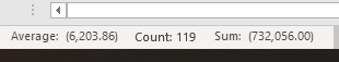 But how can the average number of days be negative? Look at row 5, the AFL-CIO again. This request doesn’t have a final date so the amount in column G is a big negative number. We can correct that. Leaving column G highlighted, click on the dropdown for column H, then on the list at the bottom unclick the check mark in the box marked (Blanks). This will filter out the requests that have no final date. Now the average response time changes to 81.56 days.
Now, try clicking on the dropdown for column G. Instead of filtering on the list of numbers, let’s try something different. Just above the list you’ll see the menu choice “Number Filters”, click on that. You’ll see some choices that you can use to look for some data. Click on Top 10, then click “OK” on the box that appears. Only the ten requests that took the longest time to finalized will display and the average time for these is 460 days. Let’s try something else. Start with nothing filtered. So, click on the dropdowns for columns G & H then click on the “Clear Filter” menu choice. You’ll notice that when the data is filtered that the row numbers on the left of the spreadsheet change to blue. When your filters are cleared, they will change back to black. Now click on the dropdown for “Request Description”. Just above the list of items there is a search box. You can type terms into that box to use as a filter. Try typing NAFTA into that box. There should be three items that pop up. You can see from playing around with this that filters can be a powerful tool to use when looking at data. Now a challenge for you. Using this spreadsheet find the following: All requests that mention “Trump”. The five requests that received the quickest responses. The final reply date that was probably an entry error. I’ll post the answers in my next entry.
0 Comments
Leave a Reply. |
|||
 RSS Feed